Big Data Management Exercises
Principle in Data Science Exercises
Data Analytics Exercises
Data Mining Exercises
Network Security Exercises
Other Exercises:
Python String Exercises
Python List Exercises
Python Library Exercises
Python Sets Exercises
Python Array Exercises
Python Condition Statement Exercises
Python Lambda Exercises
Python Function Exercises
Python File Input Output Exercises
Python Tkinter Exercises


Big Data - Exercises 3
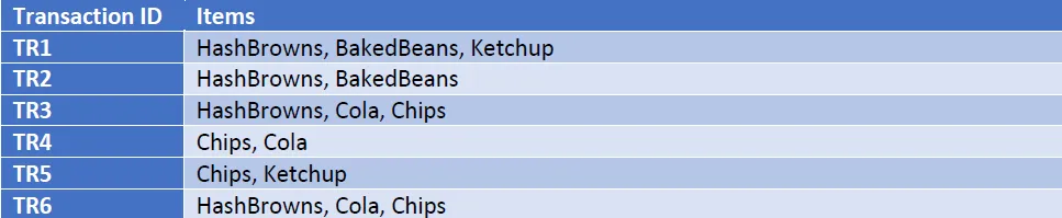
41a. Frequent Itemsets and Association RulesYou are to use the A-Priori algorithm to perform Market Basket analysis on the following transactions obtained from a shop.
The given support threshold is, s = 1/3 out of all the total number of transactions. The total number of transactions is 6. The confidence threshold is set at c = 3/5
Produce the followings:
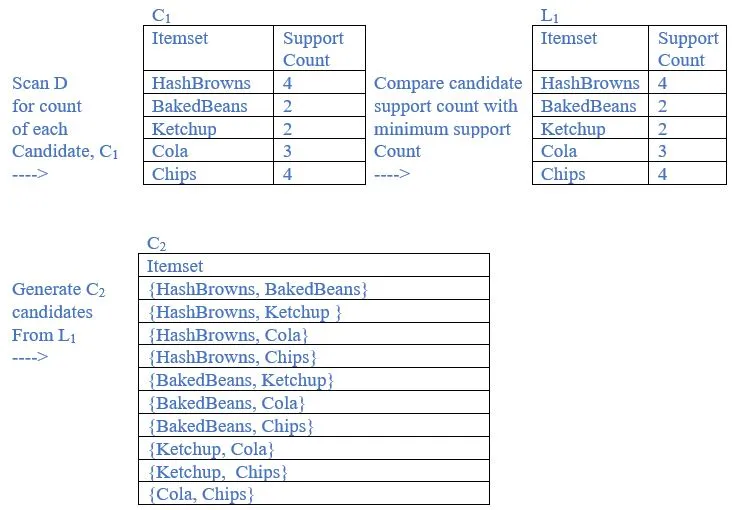
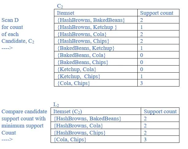
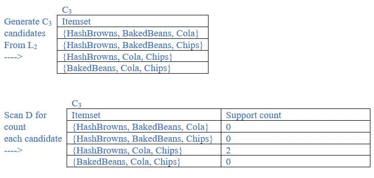
• Candidate and frequent itemsets for each scan of the database
• List all the final frequent itemsets.
• List the association rules generated and highlight the strong association rules
o Sort the association rules by its confidence value
Ans:
support threshold = 1/3
minimum support = 1/3 * 6 = 2
b. List all the final frequent itemsets.
Ans:
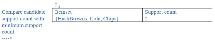
{HashBrowns}, {BakedBeans}, {Ketchup}, {Cola}, {Chips}, {HashBrowns, BakedBeans}, {HashBrowns, Cola}, {HashBrowns, Chips},{Cola, Chips}, {HashBrowns, Cola, Chips} are frequent itemsets.
c. List the association rules generated and highlight the strong association rules. Sort the association rules by its confidence value
Ans:
Generate association rule:
Based on the frequent itemset discovered in (b), the association could be
1. {HashBrowns} => {BakedBeans}
Confidence = support{HashBrowns, BakedBeans }/support {HashBrowns}
= 2/4 = 50%
2. {BakedBeans} => {HashBrowns}
Confidence = support{HashBrowns, BakedBeans }/support {BakedBeans}
= 2/2 = 100%
3. {HashBrowns} => {Cola}
Confidence = support{HashBrowns, Cola}/support {HashBrowns}
= 2/4 = 50%
4. {Cola} => {HashBrowns}
Confidence = support{HashBrowns, Cola}/support {Cola}
= 2/3 = 67%
5.{HashBrowns} => {Chips}
Confidence = support{HashBrowns, Chips}/support {HashBrowns}
= 2/4 = 50%
6. {Chips} =>{HashBrowns}
Confidence = support{HashBrowns, Chips}/support {Chips}
= 2/4 = 50%
7. {Cola} => {Chips}
Confidence = support{Cola, Chips}/support {Cola}
= 3/3 = 100%
8. {Chips}=>{Cola}
Confidence = support{Cola, Chips}/support {Chips}
= 3/4 = 75%
9. {HashBrowns, Cola} => {Chips}
Confidence = support{HashBrowns, Cola, Chips}/support {HashBrowns, Cola}
= 2/2 = 100%
10. {HashBrowns, Chips} => {Cola}
Confidence = support{HashBrowns, Cola, Chips}/support {HashBrowns, Chips}
= 2/2 = 100%
11. {Cola, Chips} => { HashBrowns}
Confidence = support{HashBrowns, Cola, Chips}/support {Cola, Chips}
= 2/3 = 67%
12. {HashBrowns} => {Cola, Chips}
Confidence = support{HashBrowns, Cola, Chips}/support {HashBrowns}
= 2/4 = 50%
13. {Cola} => {HashBrowns, Chips}
Confidence = support{HashBrowns, Cola, Chips}/support {Cola}
= 2/3 = 67%
14. {Chips} => {HashBrowns, Cola}
Confidence = support{HashBrowns, Cola, Chips}/support {Chips}
= 2/4 = 50%
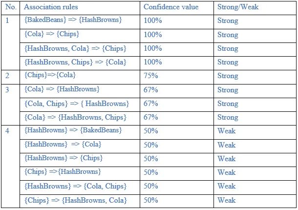
The association rules are strong if the minimum confidence threshold is 3/5 or 60%. The table below shows generated association rules with its strong association rules. The association rules also sorted by its confidence value.
42a. Import the downloaded dataset to HDFS.
Ans:
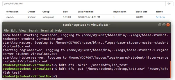
Step 1: Create a new directory as lab_test in HDFS.
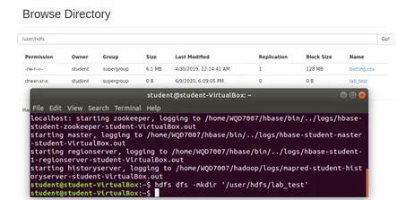
Step 2: Import a file into HDFS using the following commands.
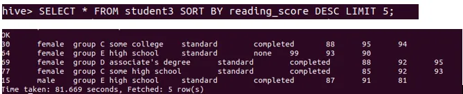
b. By using Hive, identify 5 rows of data that have the highest reading score.
Step 1: Create external hive table.
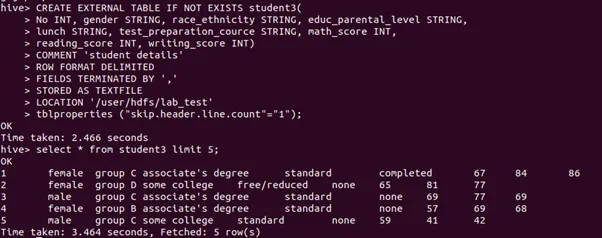
Step 2: Sort out the 5 rows that have highest reading score using the following command.
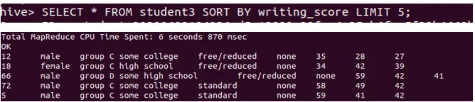
c. Identify 5 lowest Writing score using the following commands:
43a. Import text from a file to HDFS
Ans:
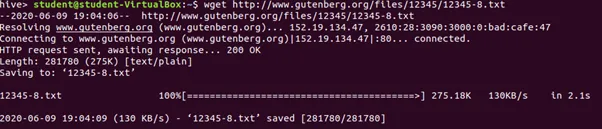
Step 1: Using wget to download and save the text file in local directory.
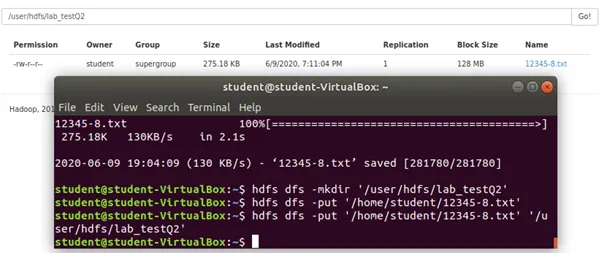
Step 2: Create a new directory as lab_testQ2 in HDFS.
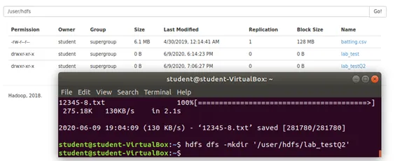
Step 3: Imported text file into HDFS using the following command (last command).
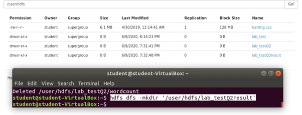
43b. Run a word count program using Hadoop MapReduce concept to count the word occurrence of the imported text as in question 18. Save the results in HDFS.
Ans:
Step 1: Create another new directory for wordcount result as lab_testQ2result using the following command.
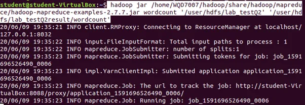
Step 2: Run the wordcount using the following command.
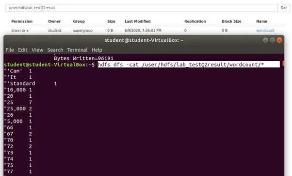
Step 3: Display the wordcount result.
43c. Import the result from 19b to Hive. Display: 5 words with highest counts in ascending alphabetical order.
Ans:
Step 1: Create an external hive table and named as wordcount
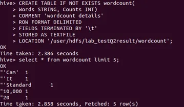
Step 2: 5 words with highest counts in ascending alphabetical order
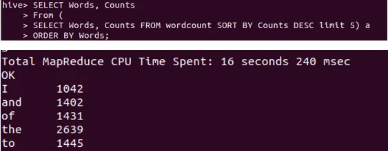
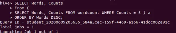
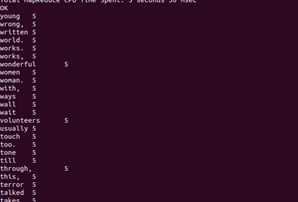
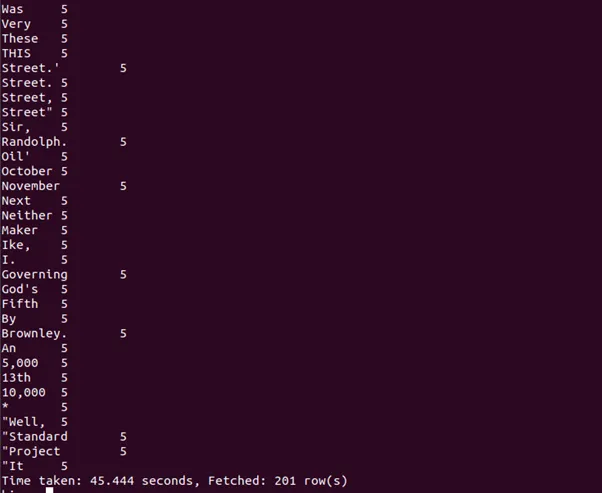
43d. Import the result from 19b to Hive. Display: 5 words with 5 counts in descending alphabetical order.
Ans:
.
.
.
.
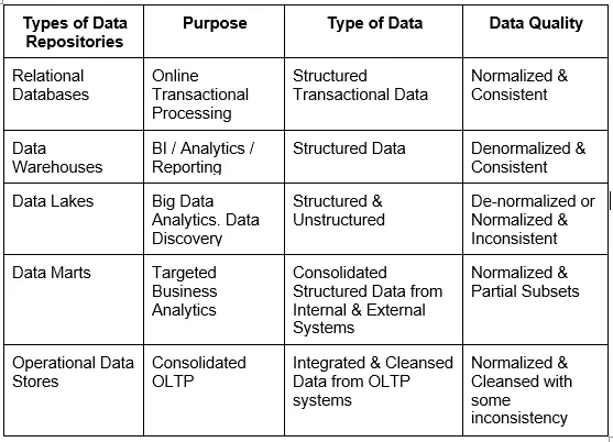
44. What are different types of data repositories?
Ans:
45. How do you compute support for items in each basket? And what is a support threshold? What are frequent itemsets?
Ans:
To compute support for items in each basket, we must sum up the number of baskets containing all the selected item. The support of the rule is the fraction of the database which contains both X and Y.
The support threshold is a minimum support, an itemset satisfies minimum support if the occurrence frequency of the itemset is greater than or equal to minimum support.
If an itemset satisfies minimum support, then it is a frequent itemset.
46. How do you evaluate an association rule? What is the difference between the confidence and the significance of an association rule?
Ans:
The association rule is evaluated based on the statistical measures such as support and confidence to the classic rule in Propositional Logic.
The confidence of an association rule X⇒Y is the proportion of the transactions containing X which also contain Y.
The significance of an association rule X⇒Y is the subtraction of confidence value from proportion of the transactions containing Y. In addition, the significance of an association rule is the absolute value of the amount by which the confidence differs from what you would expect, were items selected independently of one another.
47. What is the main limitation of the naïve algorithm for counting pairs?
Ans:
The main limitation is the huge main memory is occupied for computation process during association rule evaluation. For instance, when pairs counting process, if the main memory is not sufficient then adding 1 to a random count will most likely require us to load a page from disk. This ended up counting process has come to stop due to sufficient of main memory.
48. Here is a collection of twelve baskets. Each contains three of the six items 1 through 6.
{1, 2, 3} {2, 3, 4} {3, 4, 5} {4, 5, 6} {1, 3, 5} {2, 4, 6} {1, 3, 4} {2, 4, 5} {3, 5, 6} {1, 2, 4} {2, 3, 5} {3, 4, 6}
Suppose the support threshold is 4. On the first pass of the PCY Algorithm we use a hash table with 11 buckets, and the set {i, j} is hashed to bucket i×j mod 11.
(a) By any method, compute the support for each item and each pair of items.
Ans:

(b) Which pairs hash to which buckets?
Ans:

(c) Which buckets are frequent?
Ans:
Bucket 1, 2, 4, 8
(d) Which pairs are counted on the second pass of the PCY Algorithm?

49. Let M be the matrix of data points
Ans:

a. What are the MT M and MMT?
Ans:

b. Compute the eigenpairs for MTM
Ans:

det(A)=0 (30-λ)(354-λ)-10000=0 λ^2-384λ+620=0 λ=192±2√9061 Eigen values of M^T M are λ_1=382.379,λ_2=1.621 Eigenvector 1: For eigenvalue λ_1=382.379, the corresponding eigenvectors are calculated as follow:


c. What do you expect to be the eigenvalues of MMT?
Ans:
Since dim(MT M) < dim(MMT), the eigenvalues of MMT are eigenvalues of MTM plus additional 0’s. Thus, the eigenvalues λ' of MMT are 382.379, 1.621, 0, and 0.
d. Find the eigenvectors of MM^T using your eigenvalues from c.
Ans:
Let e be the eigenvectors:- MTMe = λe MMTMe = Mλe = λ(Me) Eigenvector of e’ of MMT are Me where e are the eigenvectors of MTM, plus eigenvectors corresponding to additional 0’s.


50a. Compute the representation of Leslie in concept space.
Ans:
qLeslie = [0 3 0 0 4]
Representation of Leslie in concept space:

50b. How do we use the representation of Leslie in concept space, to predict Leslie’s preferences for other movies in the example data? Ans:
Leslie’s preferences for other movies in the example data is predicted using the representation of Leslie in concept space by mapping it back with VT:

51. Three computers, A, B, and C, have the numerical features listed below:

We may imagine these values as defining a vector for each computer, for instance, A’s vector is [3.06, 500, 6]. We can compute the cosine distance between any two of the vectors, but if we do not scale the components, then the disk size will dominate and make differences in the other components essentially invisible.
Let us use 1 as the scale factor for processor speed, α for the disk size, and β for the main memory size.
a. In terms of α and β, compute the cosines of the angles between the vectors for each pair of the three computers.

b) A certain user has rated the three computers in Table 1, as follows: A: 4 stars, B: 2 stars, C: 5 stars.
i. Normalize the ratings for this user (use the average for normalization)
Average of the rating : (4+2+5)/3=11/3
Ans:
A: 4-11/3 = 1/3
B: 2-11/3 = -5/3
C: 5-11/3 = 4/3
ii. Compute a user profile for the user, with components for processor speed, disk size, and main memory size, based on the data
Ans:
Processor Speed : (1/3) X 3.06 + (-5/3) X 2.68 + (4/3) X 2.92 = 0.4467
Disk Size : (1/3) X 500 + (-5/3) X 320 + (4/3) X 640 = 486.6667
Main-Memory Size : (1/3) X 6 + (-5/3) X 4 + (4/3) X 6 = 3.3333
52a. Treating the utility matrix as boolean, compute the Jaccard distance between each pair of users.

Ans:
Jaccard(A,B)= 1 - 4/8 = 1/2
Jaccard(A,C)= 1 - 3/8 = 5/8
Jaccard(B,C)= 1 - 3/8 = 1/2
52b. Repeat Part (a) but use the cosine distance.
Ans:
Cosine Distance = 1 – Cosine Similarity Cosine Distance of A and B:

Cosine Distance of A and C:

Cosine Distance of B and C:

53. With regards to the architecture of a search engine, a more-like-this query occurs when the user can click on a particular document in the result list and tell the search engine to find documents that are similar to the clicked document.
Describe which low-level components are used to answer this type of query and the sequence in which they are used.
Ans:
The More Like This Query searches for documents that are similar to a given set of documents. To achieve this kind of query, the More Like This Query chooses a set of representative words from the set of input documents. Then, a query is formed using these extracted wordings. After that, the system performs the query and the results based on this newly formed query are outputted. In terms of the input, the users are responsible to control what documents to use as input, as well as how exactly the system will perform selection on the terms to be used and also the formation of the final query.
The simplest scenario is a situation where users provide a piece of texts and let the system search for documents that are similar to the texts, such as finding movie or drama documents that contain texts similar to “Magical fairy tale” in their “description” fields, at the same time setting limits for the number of selected words to be 10.
54. In reference to vector space model for ranked retrieval, compute the similarity between
• The query: “digital cameras” and
• The document “digital cameras and video cameras”
Referring to Table below, assume N = 10,000,000, use logarithmic term weighting (wf columns) for query and document, idf weighting for the query only and cosine normalization for the document only. Treat and as a stop word. Enter term counts in the tf columns. What is the final similarity score?

Ans:

Query:
Calculation for wf:
Wf for digital = 1 + log10 (1) = 1
Wf for video = 0
Wf for cameras = 1 + log10 (1) = 1
Calculation for idf:
Idf for digital = log10 (10000000/1000) = 3
Idf for video = log10 (10000000/10000) = 2
Idf for cameras = log10 (10000000/1000) = 2.3
Calculation for qi:
Qi for digital = 1 × 3 = 3
Qi for video = 0 × 2 = 0
Qi for cameras = 1 × 2.3 = 2.3
Document:
Calculation for wf:
Wf for digital = 1 + log10 (1) = 1
Wf for video = 1 + log10 (1) = 1
Wf for cameras = 1 + log10 (2) = 1.3
Calculation for di:
L2 norm = √((1^2+1^2+〖1.3〗^2 ) = 1.92
Di for digital = 1/1.92 = 0.52
Di for video = 1/1.92 = 0.52
Di for cameras = 1.3/1.92 = 0.68
Multiply qi with di:
Digital = 3 × 0.52 = 1.56
Video = 0 × 0.52 = 0
Cameras = 2.3 × 0.68 = 1.56
Final Similarity Score = 1.56 + 0 + 1.56 = 3.12
55. Table below presents the term vectors for the three novels. These are based on raw term frequency only and are normalized as if these were the only terms in the collection. (Since affection and jealous occur in all three documents, their tf-idf weight would be 0 in most formulations.)
In reference to vector space model for ranked retrieval,

a. Compute the score for the query affection for the three documents (SaS: Sense and Sensibility, PaP: Pride and Prejudice, WH: Wuthering Heights)
Ans:
Score for 3 documents = (0.996 × 0.993) + (0.996 × 0.847) + (0.993 × 0.847) = 2.67
55b. Show that (if possible) the ordering of the scores of the three documents, is the reverse for the query jealous gossip.
Ans:
For the query affection:
Score(q, SaS) = 0.996, Score(q, PaP) = 0.993, Score(q, WH) = 0.847
Order: SaS, PaP, WH
For the query jealous gossip:
Score(q, SaS) = 0.087 + 0.017 = 0.104
Score(q, PaP) = 0.120 + 0 = 0.120
Score(q, WH) = 0.466 + 0.254 = 0.72
Order: WH, PaP, SaS
Thus, the score order for query jealous gossip is the reverse order of the case for query affection. 56. 1. Perform a hierarchical clustering of the one-dimensional set of points 1, 4, 9, 16, 25, 36, 49, 64, 81, assuming clusters are represented by their centroid (average), and at each step the clusters with the closest centroids are merged.
Ans:

57a. Compute the representation of the clusters as in the BFR Algorithm. That is, compute N, SUM, and SUMSQ for each of the clusters.

Ans:
Cluster 1: (2,2), (3,4), (5,2)
N = 3
SUM = [10, 8]
SUMSQ = [38,24]
Cluster 2: (4,8), (4,10), (6,8), (7,10)
N = 4
SUM = [21, 36]
SUMSQ = [117, 328]
Cluster 3: (11,4), (12,3), (10,5), (9,3), (12, 6)
N = 5
SUM = [54, 21]
SUMSQ = [590, 95]
57b. Compute the variance and standard deviation of each cluster in each of the two dimensions.
Ans:
Cluster 1:
1st dimension
Variance in the first dimension = 〖38/3 – (10/3)〗^2 = 1.556
Standard deviation = √1.556 = 1.247
2nd dimension
Variance in the first dimension = 〖24/3 – (8/3)〗^2 = 0.889
Standard deviation = √0.889=0.943
Cluster 2:
1st dimension
Variance in the first dimension = 〖117/4 – (21/4)〗^2 = 1.6875
Standard deviation = √1.6875 = 1.299
2nd dimension
Variance in the first dimension = 〖328/4 – (36/4)〗^2 = 1
Standard deviation = √1 = 1
Cluster 3:
1st dimension
Variance in the first dimension = 〖590/5 – (54/5)〗^2 = 1.36
Standard deviation = √1.36 = 1.166
2nd dimension
Variance in the first dimension = 〖95/5 – (21/5)〗^2 = 1.36
Standard deviation = √1.36 = 1.166
57. The goal of Support Vector Machine is to fine a hyperplane, i.e., a decision boundary that linearly separates the points into different classes.
Given the hyperplane defined by y = x1 - 2x2. Find the followings:
i. Find the values of the vector w and the value for b describing the decision boundary.
Ans:
The equation for the hyperplane/ decision boundary is wTx + b = 0
And the hyperplane is defined as y = x1 - 2x2 = (1,-2)Tx
Therefore w = (1,-2) and b = 0
57ii. Evaluate whether the following points are correctly predicted.
a. y =1, x = (1,0) Ans:
x = (1,0), wTx + b = 1 and is greater than 0, therefore the label is 1.
Label predicted is y = 1.
Therefore, the labeling is correct.
57ii. Evaluate whether the following points are correctly predicted.
b. y = 1, x = (1,1)
Ans:
x = (1,1), wTx + b = -1 and is lesser than 0, therefore the label is -1.
Label predicted is y = 1.
Therefore, the labeling is incorrect.
More Free Exercises:
Data Science ExercisesBig Data Management Exercises
Principle in Data Science Exercises
Data Analytics Exercises
Data Mining Exercises
Network Security Exercises
Other Exercises:
Python String Exercises
Python List Exercises
Python Library Exercises
Python Sets Exercises
Python Array Exercises
Python Condition Statement Exercises
Python Lambda Exercises
Python Function Exercises
Python File Input Output Exercises
Python Tkinter Exercises