Big Data Management Exercises
Principle in Data Science Exercises
Data Analytics Exercises
Data Mining Exercises
Network Security Exercises
Other Exercises:
Python String Exercises
Python List Exercises
Python Library Exercises
Python Sets Exercises
Python Array Exercises
Python Condition Statement Exercises
Python Lambda Exercises
Python Function Exercises
Python File Input Output Exercises
Python Tkinter Exercises


Data Mining - Exercises 1
1. Define "Data Mining" in terms of Business Intelligence (keeping in mind the data transformation from Online Transaction Process (OLTP) to Online Analytic Process (OLAP)).Ans:Data mining is a process of discovering useful patterns from massive datasets that can contribute valuable business intelligence. The raw data from business can be converted into actionable information using data mining technique and therefore provide business intelligence. The business daily operational data is stored in online transaction processing (OLTP) systems. Hence, all the historical operational raw data can be retrieved from OLTP systems in a company. The raw data is loaded into data warehouse after subjected to Extract, Transform and Load (ETL) operations. The data reprocessing has completed after ETL operations. Then, the cleaned data in the data warehouse is ready for data analysis to help the manger in making faster and precise business decisions. The combination of data mining and online analytic process (OLAP) are used to generate report with useful patterns and business insight. Hence, it can help a manager to improve a business decision in shorter time.
2. 13, 15, 16, 16, 19, 20, 20, 21, 22, 22, 25, 25, 25, 25, 30, 33, 33, 35, 35, 35, 35, 36, 40, 45, 46, 52, 70
2(a) What is the mean of the data?
Ans: Mean = (13 + 15 + 16 + 16 + 19 + 20 + 20 + 21 + 22 + 22 + 25 + 25+ 25+ 25+ 30+ 33+ 33+ 35+ 35+ 35+ 35+ 36+ 40+ 45+ 46+ 52+ 70)/27
Mean = 29.96
2(b) What is the median?
Ans: 13, 15, 16, 16, 19, 20, 20, 21, 22, 22, 25, 25, 25, 25, 30, 33, 33, 35, 35, 35, 35, 36, 40, 45, 46, 52, 70.
Median = 25
2(c) What is the mode of the data?
Ans: Mode = 25 and 35
2(d) Use smoothing by bin means to smooth the above data, using a bin depth of 3. Illustrate your steps.
Ans: Step 1: Sort the data in ascending order.
13, 15, 16, 16, 19, 20, 20, 21, 22, 22, 25, 25, 25, 25, 30, 33, 33, 35, 35, 35, 35, 36, 40, 45, 46, 52, 70.
Step 2: Calculate the number of data in each bin with bin depth of 3.
Number of data = 27
Each bin consists of 3 data.
Bin = 9
Step 3: Calculate the mean value for each bin.
For bin 1:
(13 + 15 + 16)/3 = 14.67
For bin 2:
(16 + 19 + 20)/3 = 18.33
For bin 3:
(20 + 21 + 22)/3 = 21
For bin 4:
(22 + 25 + 25)/3 = 24
For bin 5:
(25 + 25 + 30)/3 = 26.67
For bin 6:
(33 + 33 + 35)/3 = 33.67
For bin 7:
(35+ 35+ 35)/3 =35
For bin 8:
(36 + 40 + 45)/3 = 40.33
For bin 9:
(46 + 52 + 70)/3 = 56
Step 4: Result: Smoothing by bin means
Bin 1: 14.67, 14.67, 14.67
Bin 2: 18.33, 18.33, 18.33
Bin 3: 21, 21, 21
Bin 4: 24, 24, 24
Bin 5: 26.67, 26.67¸ 26.67
Bin 6: 33.67, 33.67, 33.67
Bin 7: 35, 35, 35
Bin 8: 40.33, 40.33, 40.33
Bin 9: 56, 56, 56
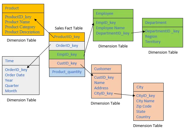
3. Suppose you have the following four Dimension Tables namely Time, Customer, Employee and Product. Construct a snowflake scheme by developing "Sales" Fact Table. The linkage attribute in the dimension tables can be used to split the table to form a snowflake scheme. The aggregate variable of fact table can be "quantity" of products.
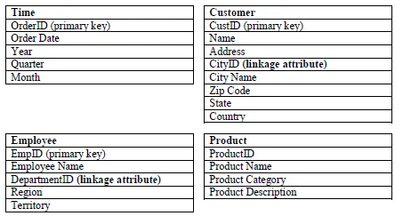
Ans:
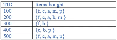
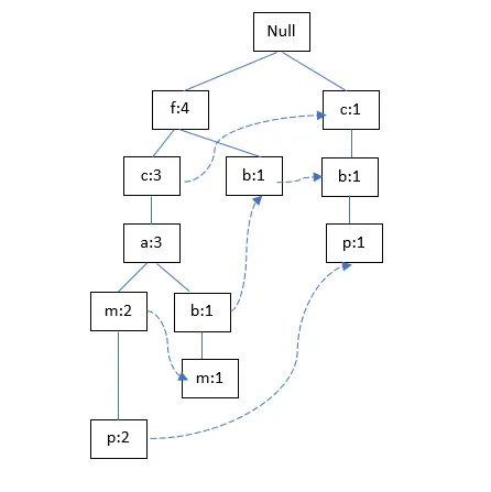
Suppose you have the following transactional database, construct an FP (frequent pattern) tree from this transaction database.
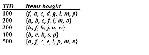
Ans:
Let us assume minimum support = 3.
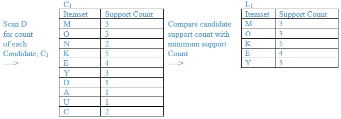
Count each item
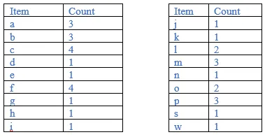
Sort the item in descending order with min support
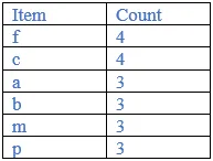
Rearrange the ordered frequent items.
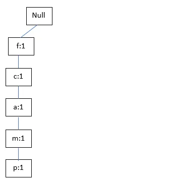
Construct FP tree
TID 100:
TID200:
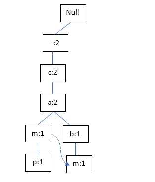
TID300:
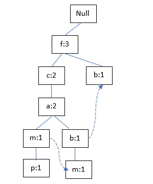
TID400:
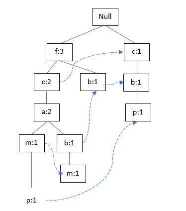
TID500:
4. Let us consider the dataset of sales related to computer systems (e.g. hardware and software) shown below. We are required to learn a decision tree which predicts the profit either up or down based on certain features i.e. condition, upgradable and type.
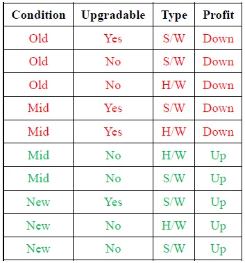
Calculate the Information Gain of feature "Condition" based on,
Entropy (Profit)
Entropy (Old)
Entropy (Mid)
Entropy (New)
Entropy (Condition)
Ans:
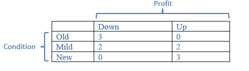
Entropy(Profit) = p+(-log2p+) + p-(-log2p-) = -[5/10*(log25/10) + 5/10*(log25/10)] = 1
Entropy(Old) = = -[3/3*(log23/3) + 0/3*(log20/3)] = 0
Entropy(Mid) = -[2/4*(log22/4) + 2/4*(log22/4)] = 0.4
Entropy(New) = -[0/3*(log20/3) + 3/3*(log23/3)] = 0
Entropy(Condition) = 0 + 0.4 + 0 = 0.4
Information Gain (Condition) = 1 – 0.4 = 0.6
6. Write down the steps of DBScan algorithm.
Ans:
Step 1: Assign value of epsilon and minimum point.
Step 2: Select a point, p from the dataset arbitrary.
Step 3: Retrieve all the points which are density-reachable from the selected point, p with respect to the value of epsilon and minimum points.
Step 4: Selected point, p is regarded as core point if satisfy the minimum points requirement. Then a cluster is formed. Or if selected point, p is a border point, no point is density-reachable from p and DBSCAN visits the next point of the dataset.
Step 5: Iterate through the unvisited points in the dataset until the points are assigned either with border or core points. Lastly, the remaining points do not belong to any core or border points are treated as noise point.
7. Select the best non-target features using one of statistical methods "correlation", "Chi-square", or "ANOVA". Your solution should describe the relevant statistical findings.
Ans:
Using Chi-square method to select the best non-target features.
• Define hypothesis with 95% confidence that is alpha = 0.05:
Null hypothesis (H0) = The variables are independent
Alternate hypothesis (H1) = The variables are not independent
• The degree of freedom = (no. of col -1)*(no. of row -1) = (7-1)*(2-1) = 6
• Chi square value can be obtained through orange 3
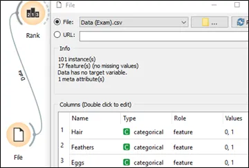
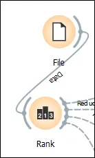
a. Import file into orange 3 and assign the type of data and its role, respectively.
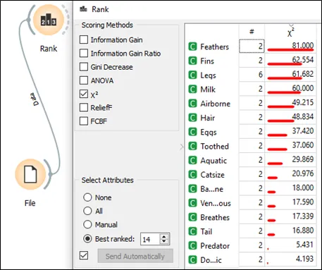
b. Link data to Rank icon.
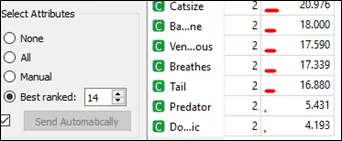
c. Tick chi square under the scoring method in the rank and the value of chi square for each feature can be seen in the following screen shot.
• Accept or reject the null hypothesis
a. With 95% confidence that is alpha = 0.05
b. degree of freedom =6
c. Hence Chi square is 12.59
d. For calculate chi square more than 12.59 are fall under rejecting null hypothesis area. So, the variables are not independent, and they can be selected for model fitting. In summary, first 14 features are rejecting null hypothesis and only 2 features accepting null hypothesis. Lastly, 14 features are selected for model training and remained only 2 features (predator and domestic) are independent variable. The higher the chi-square value, then the feature is more rely on the response, hence the feature can be selected for model fitting.
8. Using Orange 3 to do model fitting among the three algorithms (Naïve Bayes, Random Forest, and Support Vector Machine).
Step 1: Import file (Exam.csv) into Orange 3.
Step 2: Link the file with Rank to calculate chi square.
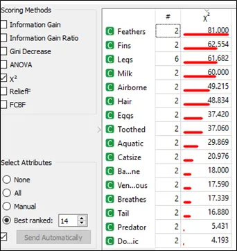
Step 3: Based on result from question (1), choose best ranked 14 in the select attributes section and tick the box with send automatically in the orange 3 as shown below:
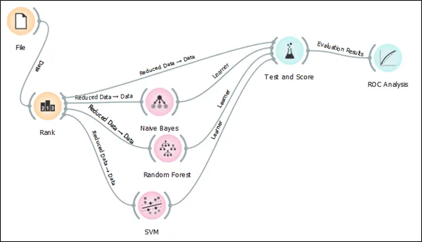
Step 4: The selected features are linked to Naïve Bayes, Random Forest, and Support Vector Machine (SVM) and test and score.
Step 5: The classification algorithms are linked to the test and score in order to generate the performance of these three models.
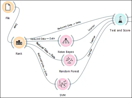
Step 6: 10-fold cross validation is selected under the sampling section. The result of three algorithms can be seen in the following screen shot.
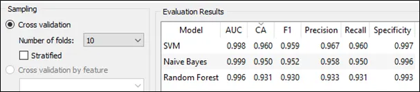
The result of three algorithms in terms of classification accuracy and false positive rate.
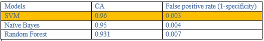
According to the result from Orange 3, the SVM able to perform the best in terms of classification accuracy and false positive rate. Hence, SVM is my choice.
9. Discuss the performance metric of all three algorithms in terms of Receiver Operator Characteristic (ROC) curve.
The test and score is connected to ROC analysis in the Orange 3 to obtain the ROC curve.
The ROC curve for target 1:
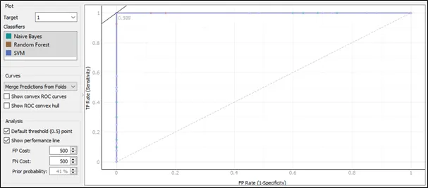
The ROC curve plots a false positive rate on x axis against true positive rate on y-axis. Based on the ROC curve for target 1, the performance for three algorithms is similar as they are having almost the same pattern in the ROC curve.
The ROC curve for target 2:
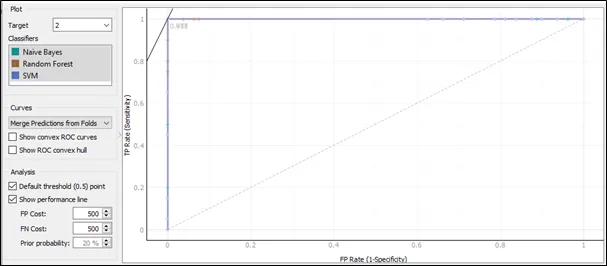
Based on the ROC curve for target 2, the performance for three algorithms is similar as they are also having almost the same pattern in the ROC curve.
The ROC curve for target 3:
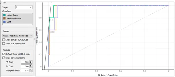
Based on the ROC curve for target 3, the performance for Naive Bayes is the best comparing to Random Forest and SVM because the curve of Naïve Bayes follows closest to the left-hand and top border of the ROC space, and this implies that the accuracy of Naïve Bayes is highest.
The ROC curve for target 4:
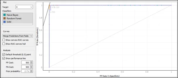
Based on the ROC curve for target 4, the Naive Bayes and Random Forest having same ROC curve pattern and they are the best result comparing to SVM because the curves of Naive Bayes and Random Forest follows closest to the left-hand and top border of the ROC space, and this implies that the accuracy of Naive Bayes and Random Forest is the highest.
The ROC curve for target 5:
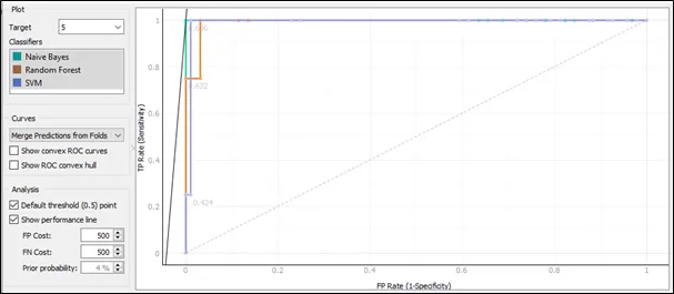
Based on the ROC curve for target 5, the performance for Naive Bayes is the best and follows by SVM because the curve of Naïve Bayes follows closest to the left-hand and top border of the ROC space, and this implies that the accuracy of Naïve Bayes is highest.
The ROC curve for target 6:
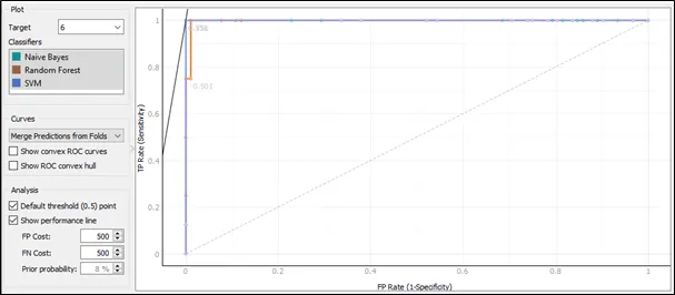
Based on the ROC curve for target 6, the Naive Bayes and SVM having same ROC curve pattern and they are the best result comparing to Random Forest because the curves of Naive Bayes and SVM follows closest to the left-hand and top border of the ROC space, and this implies that the accuracy of Naive Bayes and SVM is the highest.
The ROC curve for target 7:
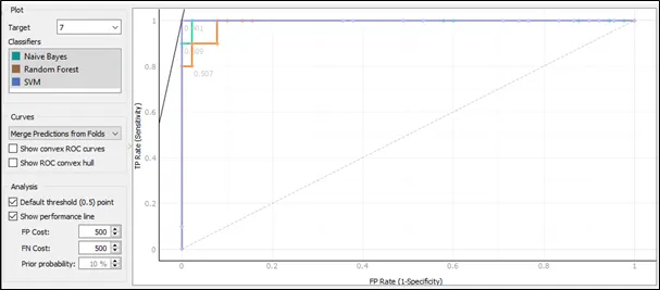
Based on the ROC curve for target 7, the performance for SVM is the best comparing to Random Forest and Naïve Bayes because the curve of SVM follows closest to the left-hand and top border of the ROC space, and this implies that the accuracy of SVM is highest.
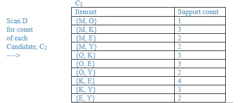
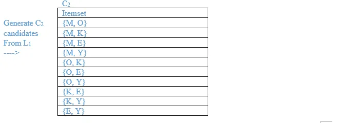
10. A database has five (5) transactions. Set min_sup = 60% and min_conf = 80%.
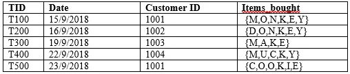
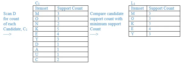
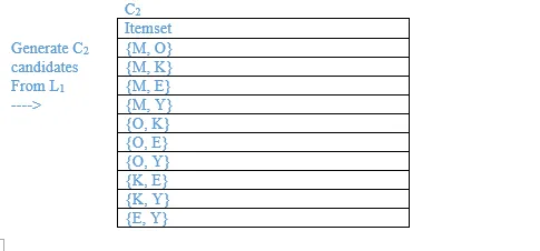
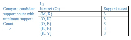
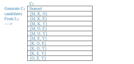
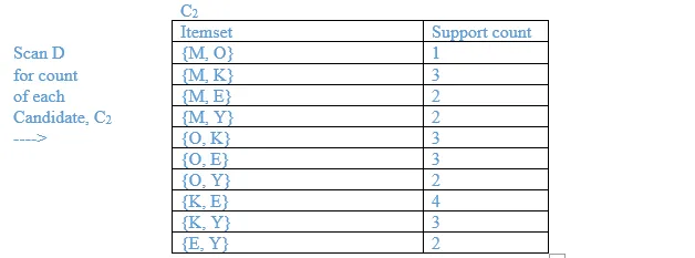
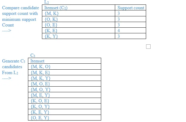
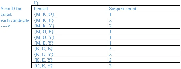
Find all frequent itemsets using Apriori. Show the candidate and frequent itemsets for each database scan. Enumerate all the final frequent itemsets. Also indicate the strong association rules that are generated.
Ans:
Minimum support = 3
Minimum confidence = 80%
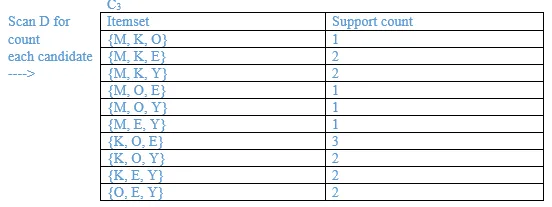
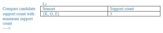
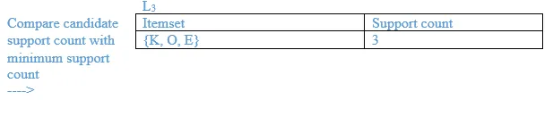
List all the final frequent itemsets.
{M}, {O}, {K}, {E}, {Y}, {M, K}, {O, K}, {O, E}, {K, E}, {K, Y}, {K, O, E}
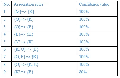
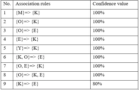
List the association rules generated and highlight the strong association rules. Sort the association rules by its confidence value
1. {M}=> {K}
Confidence = support{M, K}/support {M} = 3/3 = 100%
2. {K}=> {M}
Confidence = support{M, K}/support {K} = 3/5 = 60%
3. {O}=> {K}
Confidence = support{O, K}/support {O} = 3/3 = 100%
4. {K}=> {O}
Confidence = support{O, K}/support {K} = 3/5 = 60%
5. {O}=> {E}
Confidence = support{O, E}/support {O} = 3/3 = 100%
6. {E}=> {O}
Confidence = support{O, E}/support {E} = ¾ = 75%
7. {K}=> {E}
Confidence = support{E, K}/support {K} = 4/5 = 80%
8. {E}=> {K}
Confidence = support{E, K}/support {E} = 4/4 = 100%
9. {K}=> {Y}
Confidence = support{Y, K}/support {K} = 3/5 = 60%
10. {Y}=> {K}
Confidence = support{Y, K}/support {Y} = 3/3 = 100%
11. {K, O}=> {E}
Confidence = support{K, O, E}/support {K, O} = 3/3 = 100%
12. {K, E}=> {O}
Confidence = support{K, O, E}/support {K, E} = 3/4 = 75%
13. {O, E}=> {K}
Confidence = support{K, O, E}/support {O, E} = 3/3 = 100%
14. {K}=> {O, E}
Confidence = support{K, O, E}/support {K} = 3/5 = 60%
15. {O}=> {K, E}
Confidence = support{K, O, E}/support {O} = 3/3 = 100%
16. {E}=> {O, K}
Confidence = support{K, O, E}/support {E} = 3/4 = 75%
The association rules are strong if the minimum confidence threshold is 80%.
The table below shows generated association rules with its strong association rules.
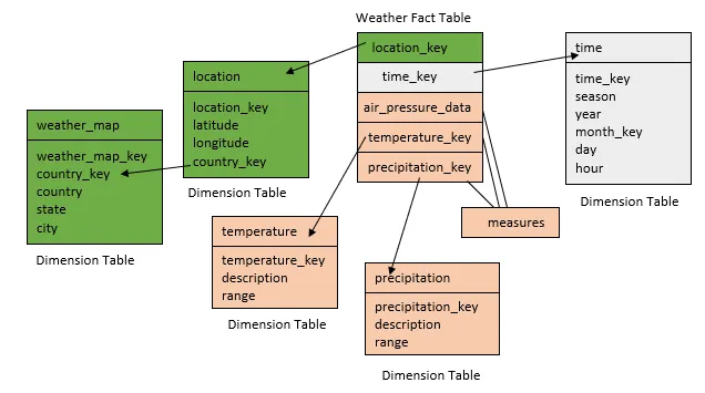
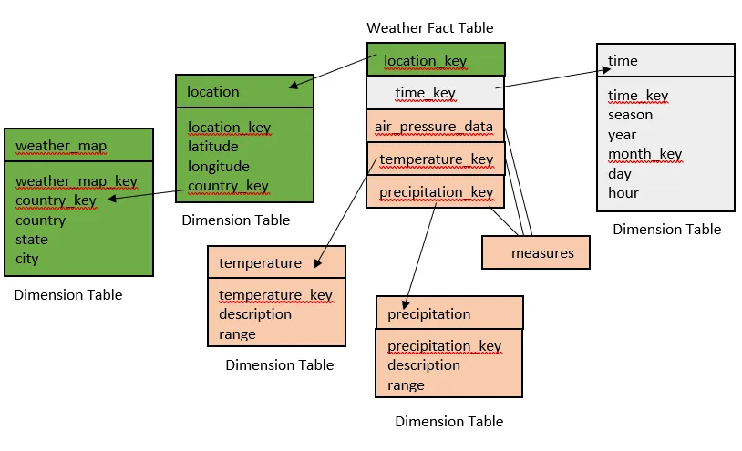
11. Design a data warehouse (implimenting snowflake schema) for a regional weather bureau. The weather bureau has about 1,000 probes, which are scattered throughout various land and ocean locations in the region to collect basic weather data, including air pressure, temperature, and precipitation at each hour. All data are sent to the central station, which has collected such data for over 10 years. Your design should facilitate efficient querying and on-line analytical processing, and derive general weather patterns in multidimensional space.
Ans:
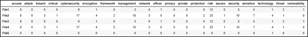
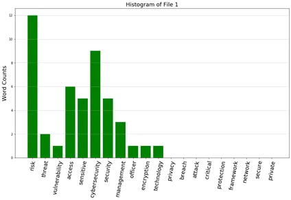
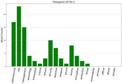
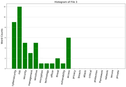
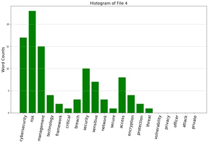
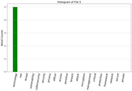
12a. Read the five source files (provided as input) in python one by one. Count the frequencies of those keywords in the source files by using the following keywords:
Keywords (20): Risk, threat, vulnerability, cybersecurity, security, privacy, officer, access, sensitive, breach, attack, encryption, technology, management, Critical, protection, framework, network, secure, private Find the frequency of each keyword in the five input files.
Ans:
import re
import pandas as pd
import numpy as np
import matplotlib.pyplot as plt

def file_opening(num):
    all_filename='File'+str(num)
    all_openfile=open(all_filename+'.txt', 'r+', encoding='utf-8')
    all_readfile=all_openfile.read()
    return(all_readfile)

def word_count(filename, num):
keywords = ['risk', 'threat', 'vulnerability', 'cybersecurity',   security','privacy', 'officer', 'access', 'sensitive', 'breach', 'attack',
            'encryption', 'technology', 'management', 'critical',
            'protection', 'framework', 'network', 'secure', 'private']

    final_word = []
    punctuations = '''!()-[]{};:'"\,<>./?@#$%^&*_~'''
    for word in filename.split():
        word = word.lower()
        for i in word:
            if i in punctuations:
                word=word.replace(i , ' ')

        words = word.split()
        for j in words:
            if j in keywords:
                final_word.append(j)

    counts = dict()
    for term in final_word[:]:
        if term in counts:
            counts[term] +=1
        else:
            counts[term] =1

    for ky in keywords:
        if ky not in counts.keys():
            counts[ky] = 0

    counts_df = pd.DataFrame(counts, index=['File'+str(num)])
    return(counts_df)

first_file = file_opening(1)
first_word_count = word_count(first_file, 1)
second_file = file_opening(2)
second_word_count = word_count(second_file, 2)
third_file = file_opening(3)
third_word_count = word_count(third_file, 3)
fourth_file = file_opening(4)
fourth_word_count = word_count(fourth_file, 4)
fifth_file = file_opening(5)
fifth_word_count = word_count(fifth_file, 5)

all = pd.concat([first_word_count, second_word_count, third_word_count, fourth_word_count, fifth_word_count])
all
12b. From question 22(a), develop five histograms of frequencies of these keywords.
Ans:
12c. Prepare a table showing the cosine similarity values of documents (no need for diagonals)
Ans:
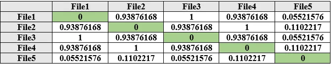
12d. Conclude which documents have highest and lowest similarity with each other
Ans:
The closer the cosine value to 1, the greater the similarity between vectors. Based on the table in (3), file 1 with file 3 have the highest similarity with each other, whileas file 2 and file 4 have the highest similarity. In contrast, file 5 with file 2 has lowest similarity with each other. Meanwhile, file 5 and file 4 has lowest similarity with each other.
13. A database has five (5) transactions. Set min_sup = 60% and min_conf = 80%.
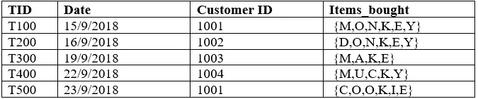
Find all frequent itemsets using Apriori. Show the candidate and frequent itemsets for each database scan. Enumerate all the final frequent itemsets. Also indicate the strong association rules that are generated.
Ans:
Minimum support = 3
Minimum confidence = 80%
List all the final frequent itemsets.
{M}, {O}, {K}, {E}, {Y}, {M, K}, {O, K}, {O, E}, {K, E}, {K, Y}, {K, O, E}
List the association rules generated and highlight the strong association rules. Sort the association rules by its confidence value
1. {M}=> {K}
Confidence = support{M, K}/support {M}
= 3/3 = 100%
2. {K}=> {M}
Confidence = support{M, K}/support {K}
= 3/5 = 60%
3. {O}=> {K}
Confidence = support{O, K}/support {O}
= 3/3 = 100%
4. {K}=> {O}
Confidence = support{O, K}/support {K}
= 3/5 = 60%
5. {O}=> {E}
Confidence = support{O, E}/support {O}
= 3/3 = 100%
6. {E}=> {O}
Confidence = support{O, E}/support {E}
= ¾ = 75%
7. {K}=> {E}
Confidence = support{E, K}/support {K}
= 4/5 = 80%
8. {E}=> {K}
Confidence = support{E, K}/support {E}
= 4/4 = 100%
9. {K}=> {Y}
Confidence = support{Y, K}/support {K}
= 3/5 = 60%
10. {Y}=> {K}
Confidence = support{Y, K}/support {Y}
= 3/3 = 100%
11. {K, O}=> {E}
Confidence = support{K, O, E}/support {K, O}
= 3/3 = 100%
12. {K, E}=> {O}
Confidence = support{K, O, E}/support {K, E}
= 3/4 = 75%
13. {O, E}=> {K}
Confidence = support{K, O, E}/support {O, E}
= 3/3 = 100%
14. {K}=> {O, E}
Confidence = support{K, O, E}/support {K}
= 3/5 = 60%
15. {O}=> {K, E}
Confidence = support{K, O, E}/support {O}
= 3/3 = 100%
16. {E}=> {O, K}
Confidence = support{K, O, E}/support {E}
= 3/4 = 75%
The association rules are strong if the minimum confidence threshold is 80%. The table below shows generated association rules with its strong association rules.
14. Design a data warehouse (implimenting snowflake schema) for a regional weather bureau. The weather bureau has about 1,000 probes, which are scattered throughout various land and ocean locations in the region to collect basic weather data, including air pressure, temperature, and precipitation at each hour. All data are sent to the central station, which has collected such data for over 10 years. Your design should facilitate efficient querying and on-line analytical processing, and derive general weather patterns in multidimensional space.
{Hint for Question 14:}
Since the weather bureau has about 1,000 probes scattered throughout various land and ocean locations, we need to construct a spatial data warehouse so that a user can view weather patterns on a map by month, by region, and by different combinations of temperature and precipitation, and can dynamically drill down or roll up along any dimension to explore desire patterns.
Ans:
More Free Exercises:
Data Science ExercisesBig Data Management Exercises
Principle in Data Science Exercises
Data Analytics Exercises
Data Mining Exercises
Network Security Exercises
Other Exercises:
Python String Exercises
Python List Exercises
Python Library Exercises
Python Sets Exercises
Python Array Exercises
Python Condition Statement Exercises
Python Lambda Exercises
Python Function Exercises
Python File Input Output Exercises
Python Tkinter Exercises